


Determination of Road Size or Capacity Based on Highway
There are two differing approaches to determining the capacity of a highway. The first, which can be termed the ‘level of service’ approach, involves establishing, from the perspective of the road user (driver), the quality of service delivered by a highway at a given rate of vehicular flow per lane of traffic. The methodology is predominant in the United States of America (US) and other countries.
The second approach, used in Britain, puts forward practical capacities for roads of various sizes and width carrying different types of traffic. Within this method, economic assessments are used to indicate the lower border of a flow range, the level at which a given road width is likely to be preferable to a narrower one. An upper limit is also arrived at using both economic and operational assessments. Together these boundaries indicate the maximum flow that can be accommodated by a given carriageway width under given traffic conditions. The first approach would be discussed in this article.
To determine the appropriate size of a road, two things are required: the desired level of service of the road as well as the estimated design traffic volume for the road.
Design Steps
Step 1: Determination of the Peak Hour Traffic
The peak hour traffic from the traffic analysis is first determined. This is known as the Design hourly volume (DHV).
![]()

Where:
Ki = ith highest annual hourly volume of traffic (in US, the 30th highest hourly volume, K30 is often used. However, values in most cases can be selected between K10 and K50). K30 implies that the road will be over capacity 29 hours per year or the hourly volume that will be reached only thirty times or exceeded only 29 times in a year and all other hourly volume of the year will be less than this value. This value constitutes better utilization of economic resources. K30 has a unique value of 0.12
Step 2: Determination of Directional Factor, D
Directional factor (D-factor) is the traffic volume proportion moving in the higher volume direction during the peak hour to the combined volume in both directions. It is usually expressed as a percentage. It represents the directional distribution of hourly traffic volumes. D30 represents the traffic volume proportion in the 30th highest hourly volume of the year traveling in the peak direction. 30th highest hourly volume for a given year is typically used for the purposes of calculating D-factor. D-factor is based on the fact that traffic volumes may not be evenly split in both travel directions during the design hour. A road located in an urban center often has equal traffic volumes in both directions, i.e., a D-factor of nearly 50%. On the other hand, a road in suburban areas carry imbalanced directional flows due to larger traffic traveling toward an urban area in the morning and away from an urban area in the evening. D-factor is determined using the expression below.


Step 3: Determination of the DDHV
Directional Design-Hour Volume (DDHV) with unit of vehicles per hour (vph) is the proportion of AADT in the peak-hour (design hour) in the predominant direction of traffic flow. DDHV is determined from field measurements on the facility under consideration or on parallel and similar facilities. It is given by multiplying AADT by K-factor and D-factor. Neither the AADT nor the ADT indicates the variations in traffic volumes that occur during the day, specifically high traffic volumes that occur during the peak hour of travel. Therefore, AADT or ADT should be adjusted for peak-hour volume and directionality, which is the purpose of calculating DDHV. DDHV is a critical design volume with a directional component. Determination of DDHV was important because designing a facility with too much capacity will be uneconomical, and a facility with too little capacity will be inadequate.
![]()

[Recall that AADT is usually determined from traffic count]
Step 4: Determination of Peak Hour Flow
Peak Hour Flow (PHF) is a measure of traffic demand variation within the analysis hour and describes the relationship between full hourly volume and the peak 15-min flow rate within the hour. It is given by dividing the hourly volume by the peak 15-min flow rate within the analysis hour. In estimating PHF, 15-min is used because it is considered as the minimum time period over which traffic flow is statistically stable. PHF is an important variable for facility design and capacity analysis because the design should always seek to accommodate the traffic demand in most peak-hour periods of the year.
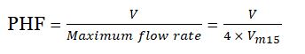

Where:
V = hourly volume in veh/h within a 24-hour period
Vm15 = maximum volume during the peak 15-min of the analysis period (veh/15-min)
Step 5: Determination of Service flow or Free flow speed
Level of service (LOS) is a quality measure describing operational conditions within a traffic stream, generally in terms of such service measures as speed and travel time, freedom to manoeuver, traffic interruptions, and comfort and convenience. Six LOS are defined for each type of facility that has analysis procedures available. Letters designate each level, from A to F.
Service A: This represents free-flow conditions where traffic flow is virtually zero. Only the geometric design features of the highway, therefore, limit the speed of the car. Comfort and convenience levels for road users are very high as vehicles have almost complete freedom to manoeuvre.
Service B: Represents reasonable free-flow conditions. Comfort and convenience levels for road users are still relatively high as vehicles have only slightly reduced freedom to manoeuvre. Minor accidents are accommodated with ease although local deterioration in traffic flow conditions would be more discernible than in service A.
Service C: Delivers stable flow conditions. Flows are at a level where small increases will cause a considerable reduction in the performance or ‘service’ of the highway. There are marked restrictions in the ability to manoeuvre and care is required when changing lane. While minor incidents can still be absorbed, major incidents will result in the formation of queues. The speed chosen by the driver is substantially affected by that of the other vehicles. Driver comfort and convenience have decreased perceptibly at this level.
Service D: The highway is operating at high-density levels but stable flow still prevails. Small increases in flow levels will result in significant operational difficulties on the highway. There are severe restrictions on a driver’s ability to manoeuvre, with poor levels of comfort and convenience.
Service E: Represents the level at which the capacity of the highway has been reached. Traffic flow conditions are best described as unstable with any traffic incident causing extensive queuing and even breakdown. Levels of comfort and convenience are very poor and all speeds are low if relatively uniform.
Service F: Describes a state of breakdown or forced flow with flows exceeding capacity. The operating conditions are highly unstable with constant queuing and traffic moving on a ‘stop-go’ basis.
Free flow is considered as a base parameter to calculate various other traffic parameters including but not limited to speed, capacity, travel time index, and planning time index. It is the speed at which free-flow traffic prevail. Free-flow speed is also the speed at which vehicles’ speeds are unaffected by surrounding conditions and other vehicles. Free-flow speed is the key parameter in estimation of freeway and multilane highway capacity.


Free flow determined above is usually considered the maximum service flow, SFmax (i)
Step 6: Determination of the Level of Service of the Road
The level of service of the road is expressed as a ratio of flow (v) to capacity (c) and usually expressed as (v/c). It is determined by the expression below:


Where:
Cj = capacity of standard highway lane for a given design speed j. For 70 km/h, 60 km/h and 50 km/h design speeds, Cj has values of 2000 v/h, 2000 v/h and 1900 v/h respectively. Table directly below shows the variation of (v/c) with level of service based on different design speed.
| Level of Service | v/c (C70) | v/c (C60) | v/c (C50) |
| A | 0.36 | 0.33 | – |
| B | 0.54 | 0.50 | 0.45 |
| C | 0.71 | 0.65 | 0.60 |
| D | 0.87 | 0.80 | 0.76 |
| E | 1.0 | 1.00 | 1.00 |
| F | variable | variable | variable |
Step 7: Determination of the Number of Lanes, N
The number of lanes, N is determined with the expression below:


Where:
fHV = heavy vehicles adjustment factor
fp = drivers familiarity adjustment factor


Where:
PT – Percentage of trucks in traffic stream
PB – Percentage of buses in traffic stream
PR – Percentage of recreational vehicles (RVs) in traffic stream.
The passenger car equivalent (pce), or the number of equivalent private cars that would occupy the same quantity of road space, for each of the above types of heavy vehicle is primarily dependent on the terrain of the highway under examination, with steep gradients magnifying the performance constraints of the heavy vehicles. The pce’s for trucks (ET), buses (EB), and recreational vehicles (ER), are defined for three different classes of terrain as shown in the Table below.
|
Types of Terrain |
|||
| Correction Factor | Level | Rolling | Mountainous |
| ET for trucks | 1.7 | 4.0 | 8.0 |
| EB for buses | 1.5 | 3.0 | 5.0 |
| ER for RVs | 1.6 | 3.0 | 4.0 |
Fp has a value of 1.0 for regular weekday commuters and a value of 0.9 – 0.75 for other classes of drivers.
Thanks
References
Rogers, M. (2003). Highway Engineering, Blackwell Publishing Limited, UK
US Department of Transportation (2018). Traffic Data Computation Pocket Guide. Federal Highway Administration
The Highway Capacity Manual (2000). Transportation research Board, National Research Council, USA.


